ML Algorithms in Numpy and PyTorch

• The goal of this is to practice building basic ML algorithms from scratch in numpy/PyTorch. I use Machine Learning from Scratch series as a starting point, generally watching the first part of the video to review the setup, then building the algorithms out myself, looking at the repo for test cases/if stuck.

import numpy as np
np.random.seed(42)
import matplotlib.pyplot as plt
import torch
import torch.nn as nn
from sklearn import datasets
from sklearn.model_selection import train_test_split
from matplotlib.colors import ListedColormap
import collections
from sklearn.datasets import make_blobs
from time import perf_counter

KNN

• Predict the class based on the most common class among the k nearest neighbors
• fit: doesn’t actually “train” the model in a traditional sense, just stores the training data.
• predict: for each point, find k nearest neighbors, then find most common class among these.

class KNN:
    def __init__(self,k=3):
        self.k = k

    def _dist(self,x1,x2):
        return np.sqrt(np.sum((x1-x2)**2))
    
    def fit(self,X,y):
        self.X_train = X
        self.y_train = y

    def _predict(self,x,debug=False):
        dists=np.array([self._dist(x,x_train) for x_train in self.X_train])
        sorted_indices = np.argsort(dists)[:self.k]
        labels = [self.y_train[i] for i in sorted_indices]
        most_common_labels = collections.Counter(labels).most_common(1)[0][0]
        if debug: 
            print("ORIGINAL: ",dists)
            print("LABELS: ",labels)
            print("MOST COMMON LABEL: ", most_common_labels)
        return most_common_labels
    
    def predict(self,X,debug):
        # X can have multiple samples, so predict for each one
        out = np.array([self._predict(x,debug) for x in X])
        if debug: print(out)
        return out

iris = datasets.load_iris()
X,y = iris.data, iris.target

X_train, X_test, y_train, y_test = train_test_split(X,y,test_size=0.2,random_state=42)
def accuracy(y_true,y_pred):
    return np.sum(y_true==y_pred)/len(y_true)


k = 3
clf = KNN(k)
clf.fit(X_train,y_train)
predictions  = clf.predict(X_test,debug=False)
print("Accuracy: ", accuracy(y_test,predictions))

Accuracy:  1.0

• First implement a naive implementation by directly converting numpy arrays to torch.tensors and replacing numpy functions with PyTorch functions.

class KNNTorchNaive:
    def __init__(self,k=3):
        self.k = k

    def _dist(self,x1,x2):
        return torch.sqrt(torch.sum((x1-x2)**2))
    
    def fit(self,X,y):
        self.X_train = X
        self.y_train = y

    def _predict(self,x,debug=False):
        dists=torch.tensor([self._dist(x,x_train) for x_train in self.X_train])
        sorted_indices = torch.argsort(dists)[:self.k]
        labels = [self.y_train[i] for i in sorted_indices]
        most_common_labels = collections.Counter(labels).most_common(1)[0][0]
        if debug: 
            print("ORIGINAL: ",dists)
            print("LABELS: ",labels)
            print("MOST COMMON LABEL: ", most_common_labels)
        return most_common_labels
    
    def predict(self,X,debug):
        # X can have multiple samples, so predict for each one
        out = torch.tensor([self._predict(x,debug) for x in X])
        if debug: print(out)
        return out

k = 3
X = torch.from_numpy(X).float()
y = torch.from_numpy(y).long()
X_train, X_test, y_train, y_test = train_test_split(X,y,test_size=0.2, random_state=42)
def accuracy(y_true,y_pred): return torch.sum(y_true==y_pred).item()/len(y_true)
clf = KNNTorchNaive(k)
clf.fit(X_train,y_train)
predictions  = clf.predict(X_test,debug=False)
print("Accuracy: ", accuracy(y_test,predictions))

Accuracy:  1.0

X_train.shape

torch.Size([120, 4])

class KNNTorchBroadcast:
    def __init__(self,k=3):
        self.k = k
    
    def fit(self,X,y):
        self.X_train = X
        self.y_train = y

    def _predict(self,x,debug=False):
        #print(x.shape)
        dists = torch.sqrt(torch.sum((self.X_train-x)**2,dim=1))
        sorted_indices = torch.argsort(dists)[:self.k]
        labels = [self.y_train[i] for i in sorted_indices] #could perhaps be optimized, but trying to keep this consistent with collections.Counter
        most_common_labels = collections.Counter(labels).most_common(1)[0][0]
        if debug: 
            print("ORIGINAL: ",dists)
            print("LABELS: ",labels)
            print("MOST COMMON LABEL: ", most_common_labels)
        return most_common_labels
    
    def predict(self,X,debug):
        # X can have multiple samples, so predict for each one
        out = torch.tensor([self._predict(x,debug) for x in X])
        if debug: print(out)
        return out

• Broadcasting in PyTorch follows these rules:

1. If the two tensors differ in the number of dimensions, the shape of the tensor with fewer dimensions is padded with ones on its leading (left) side.

2. If the shape of the two tensors does not match in any dimension, the tensor with shape equal to 1 in that dimension is stretched to match the other shape.

3. If in any dimension the sizes disagree and neither is equal to 1, an error is raised.

• We subtract tensor x of shape [4] from a tensor self.X_train of shape [120, 4], PyTorch automatically broadcasts x to the shape of self.X_train by repeating it along the 0th dimension.
  • In the dists calculation, the tensors differ in number of dimensions, so x is padded on the left with 1, becoming [1,4] according to Rule 1. Then by Rule 2, this resulting tensor is “stretched out” along 0th dimension from shape [1,4] to [120,4].

def accuracy(y_true,y_pred): return torch.sum(y_true==y_pred).item()/len(y_true)
clf = KNNTorchBroadcast(k)
clf.fit(X_train,y_train)
predictions  = clf.predict(X_test,debug=False)
print("Accuracy: ", accuracy(y_test,predictions))

Accuracy:  1.0

K-Means Clustering

• Cluster an unlabeled data set into K clusters.
  • Initialize cluster centroids randomly
  • Repeat until convergence
    • Update cluster labels, assigning points to nearest cluster centroid
    • Update cluster centroids, setting them to the mean of each cluster

class KMeans:
    def __init__(self, K, max_iters, plot_steps):
        self.K = K
        self.max_iters = max_iters
        self.plot_steps = plot_steps
        # list of lists of indices for each cluster
        self.clusters = [[] for _ in range(self.K)]
        # mean feature vector for each cluster
        self.centroids = []
        self.tol = 1e-20
    def _dist(self,x1,x2):
        return np.sqrt(np.sum((x1-x2)**2))
    # just need predict since unsupervised with no labels
    def predict(self,X,debug=False):
        self.X = X #just need for plotting
        self.n_samples, self.n_features = X.shape
        # initialize cluster centroids randomly
        self.centroids =[self.X[idx] for idx in np.random.choice(self.n_samples, size=self.K, replace=False)]
        if debug: print('init centroids: ', self.centroids); print('init clusters: ',self.clusters)
        for it in range(self.max_iters):
            # Re-initialize the clusters since else will keep appending to old ones!!! (IMPORTANT)
            self.clusters = [[] for _ in range(self.K)]
            old_centroids = np.copy(self.centroids) #else will point to self.centroids even when those are re-initialized! (IMPORTANT)
            # Update cluster labels, assigning points to nearest cluster centroid
            for i in range(self.n_samples):
                cluster_idx = np.argmin([self._dist(self.X[i,:],centroid) for centroid in self.centroids])
                self.clusters[cluster_idx].append(i)
            # Update cluster centroids, setting them to the mean of each cluster
            for i,cluster in enumerate(self.clusters):
                self.centroids[i] = np.mean([self.X[idx] for idx in cluster], axis = 0)
                
            if debug: print('centroids: ', self.centroids); print('clusters: ',self.clusters)
            if np.all([self._dist(old_centroids[i], self.centroids[i]) < self.tol for i in range(self.K)]):
                print(f'converged in {it} iterations, breaking'); break
        
    def plot(self):
        """From https://github.com/patrickloeber/MLfromscratch/blob/master/mlfromscratch/kmeans.py"""
        fig, ax = plt.subplots(figsize=(12, 8))

        for i, index in enumerate(self.clusters):
            point = self.X[index].T
            ax.scatter(*point)

        for point in self.centroids:
            ax.scatter(*point, marker="x", color="black", linewidth=2)

        plt.show()

start_time=perf_counter()
X, y = make_blobs(
    centers=3, n_samples=5000, n_features=2, shuffle=True, random_state=40
)
print(X.shape)

clusters = len(np.unique(y))
print(clusters)

k = KMeans(K=clusters, max_iters=150, plot_steps=True)
y_pred = k.predict(X,debug = False)
end_time = perf_counter()
print(f"Time taken: {end_time-start_time}")
k.plot()

(5000, 2)
3
converged in 8 iterations, breaking
Time taken: 0.36868009900172183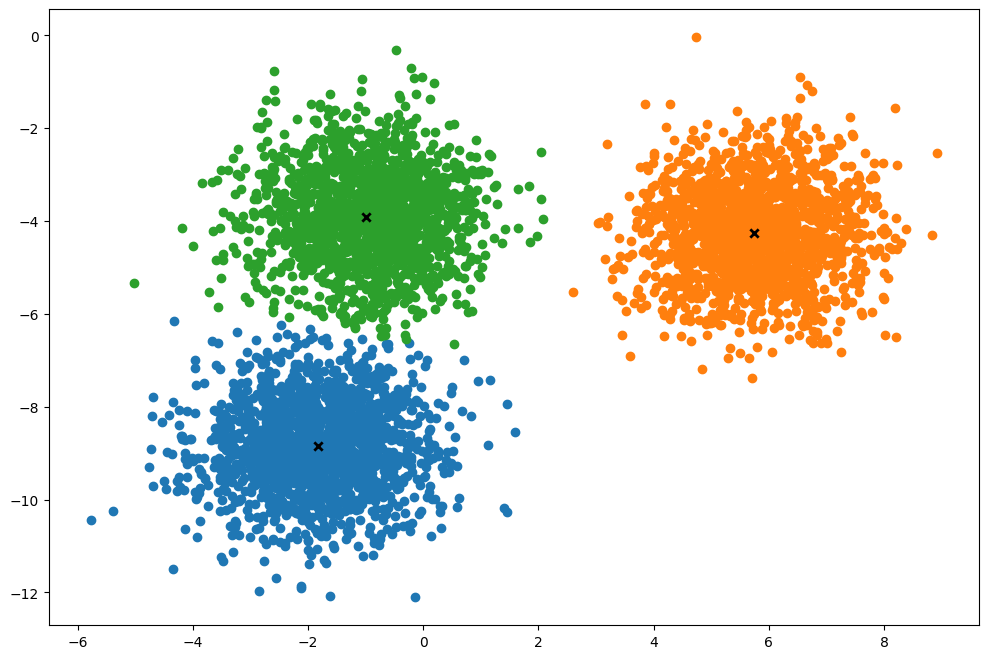

class KMeansVectDist:
    def __init__(self, K, max_iters, plot_steps):
        self.K = K
        self.max_iters = max_iters
        self.plot_steps = plot_steps
        self.clusters = [[] for _ in range(self.K)]
        self.centroids = []
        self.tol = 1e-20

    def predict(self, X, debug=False):
        self.X = X
        self.n_samples, self.n_features = X.shape
        self.centroids = self.X[np.random.choice(self.n_samples, size=self.K, replace=False)]

        for it in range(self.max_iters):
            self.clusters = [[] for _ in range(self.K)]
            old_centroids = np.copy(self.centroids)

            distances = np.sqrt(((self.X - self.centroids[:, np.newaxis])**2).sum(axis=2))
            closest_clusters = np.argmin(distances, axis=0)
            for i in range(self.n_samples):
                self.clusters[closest_clusters[i]].append(i)

            for i, cluster in enumerate(self.clusters):
                self.centroids[i] = self.X[cluster].mean(axis=0)

            if np.all(np.sqrt(np.sum((old_centroids - self.centroids) ** 2, axis=1)) < self.tol):
                print(f'converged in {it} iterations, breaking')
                break
    def plot(self):
        """From https://github.com/patrickloeber/MLfromscratch/blob/master/mlfromscratch/kmeans.py"""
        fig, ax = plt.subplots(figsize=(12, 8))

        for i, index in enumerate(self.clusters):
            point = self.X[index].T
            ax.scatter(*point)

        for point in self.centroids:
            ax.scatter(*point, marker="x", color="black", linewidth=2)

        plt.show()

start_time=perf_counter()
X, y = make_blobs(
    centers=3, n_samples=5000, n_features=2, shuffle=True, random_state=40
)
print(X.shape)

clusters = len(np.unique(y))
print(clusters)

k = KMeansVectDist(K=clusters, max_iters=150, plot_steps=True)
y_pred = k.predict(X,debug = False)
end_time = perf_counter()
print(f"Time taken: {end_time-start_time}")
k.plot()

(5000, 2)
3
converged in 7 iterations, breaking
Time taken: 0.0077601640005013905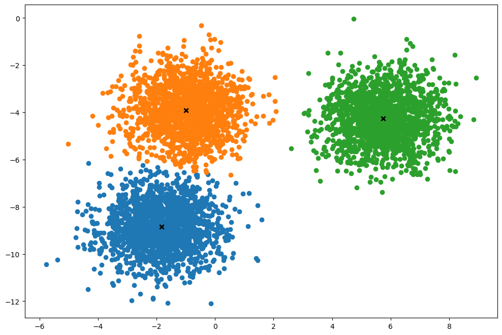

• torch.tensor() vs torch.stack(): The torch.tensor() function is used to create a new tensor, while torch.stack() is used to concatenate a sequence of tensors along a new dimension.

  In our case, [torch.mean(self.X[cluster], axis=0) for cluster in self.clusters] is a list of tensors. Each tensor is the mean of the data points in a cluster.

  If we use torch.tensor() on this list, it will try to create a new tensor that contains these tensors, which is not allowed because all elements within a tensor must be of the same type and tensors cannot contain other tensors.

  On the other hand, torch.stack() takes this list of tensors and concatenates them along a new dimension to create a single tensor. This is why torch.stack() is used in this case.

  In short, torch.stack() is used to combine existing tensors into a larger tensor, while torch.tensor() is used to create a new tensor.

class KMeansTorchNaive:
    def __init__(self, K, max_iters, plot_steps):
        self.K = K
        self.max_iters = max_iters
        self.plot_steps = plot_steps
        # list of lists of indices for each cluster
        self.clusters = [[] for _ in range(self.K)]
        # mean feature vector for each cluster
        self.centroids = []
        self.tol = 1e-20
    def _dist(self,x1,x2):
        return torch.sqrt(torch.sum((x1-x2)**2))
    # just need predict since unsupervised with no labels
    def predict(self,X,debug=False):
        self.X = X #just need for plotting
        self.n_samples, self.n_features = X.shape
        # initialize cluster centroids randomly
        #self.centroids =[self.X[idx] for idx in torch.random.choice(self.n_samples, size=self.K, replace=False)]
        self.centroids = self.X[torch.randperm(self.n_samples)[:self.K]]

        if debug: print('init centroids: ', self.centroids); print('init clusters: ',self.clusters)
        for it in range(self.max_iters):
            # Re-initialize the clusters since else will keep appending to old ones!!! (IMPORTANT)
            self.clusters = [[] for _ in range(self.K)]
            old_centroids = self.centroids.clone()
            # Update cluster labels, assigning points to nearest cluster centroid
            for i in range(self.n_samples):
                cluster_idx = torch.argmin(torch.tensor(torch.tensor([self._dist(self.X[i,:],centroid) for centroid in self.centroids])))
                self.clusters[cluster_idx].append(i)
            # Update cluster centroids, setting them to the mean of each cluster
            # for i,cluster in enumerate(self.clusters):
            #     self.centroids[i] = torch.mean(torch.tensor([self.X[idx] for idx in cluster]))
            self.centroids = torch.stack([torch.mean(self.X[cluster], axis=0) for cluster in self.clusters])
            if debug: print('centroids: ', self.centroids); print('clusters: ',self.clusters)
            if torch.all(torch.sqrt(torch.sum((self.centroids-old_centroids)**2,dim=1)) < self.tol): 
            #if np.all([self._dist(old_centroids[i], self.centroids[i]) < self.tol for i in range(self.K)]):
                print(f'converged in {it} iterations, breaking'); break
            # if torch.all([self._dist(old_centroids[i], self.centroids[i]) < self.tol for i in range(self.K)]):
            #     print(f'converged in {it} iterations, breaking'); break
        
    def plot(self):
        """From https://github.com/patrickloeber/MLfromscratch/blob/master/mlfromscratch/kmeans.py"""
        fig, ax = plt.subplots(figsize=(12, 8))

        for i, index in enumerate(self.clusters):
            point = self.X[index].T
            ax.scatter(*point)

        for point in self.centroids:
            ax.scatter(*point, marker="x", color="black", linewidth=2)

        plt.show()

start_time = perf_counter()
X, y = make_blobs(
    centers=3, n_samples=5000, n_features=2, shuffle=True, random_state=40
)
X, y = torch.tensor(X), torch.tensor(y)
print(X.shape)

clusters = len(np.unique(y))
print(clusters)

k = KMeansTorchNaive(K=clusters, max_iters=150, plot_steps=True)
y_pred = k.predict(X,debug = False)
end_time = perf_counter()
print(f"Time taken: {end_time-start_time}")
k.plot()

torch.Size([5000, 2])
3

/tmp/ipykernel_8198/1886197135.py:29: UserWarning: To copy construct from a tensor, it is recommended to use sourceTensor.clone().detach() or sourceTensor.clone().detach().requires_grad_(True), rather than torch.tensor(sourceTensor).
  cluster_idx = torch.argmin(torch.tensor(torch.tensor([self._dist(self.X[i,:],centroid) for centroid in self.centroids])))

converged in 5 iterations, breaking
Time taken: 0.8377222439994512

• OK, naive PyTorch implementation took a bit longer than basic numpy implementation.

class KMeansTorch:
    def __init__(self, K, max_iters, plot_steps):
        self.K = K
        self.max_iters = max_iters
        self.plot_steps = plot_steps
        self.tol = 1e-20


    def predict(self, X, debug=False):
        self.X = X  # just need for plotting
        self.n_samples, self.n_features = X.shape
        # initialize cluster centroids randomly
        self.centroids = self.X[torch.randperm(self.n_samples)[:self.K]]

        if debug:
            print('init centroids: ', self.centroids)

        for it in range(self.max_iters):
            old_centroids = self.centroids.clone()

            # Calculate distances from each point to each centroid
            distances = torch.cdist(self.X, self.centroids)
            if debug: print(f"distances of shape {distances.shape}: {distances}")
            # Find closest centroids
            closest_centroids = torch.argmin(distances, dim=1) #eg, shape (5000,3)-> want to find min along dim=1
            if debug: print(f"closest centroids: {closest_centroids}")
            if debug: print(f"torch.nonzero(closest_centroids == 1, as_tuple=True): {torch.nonzero(closest_centroids == 1, as_tuple=True)}")
            # Update clusters using advanced indexing
            self.clusters = [torch.nonzero(closest_centroids == i, as_tuple=True)[0] for i in range(self.K)]
            
            # Calculate new centroids
            self.centroids = torch.stack(
                [self.X[cluster].mean(dim=0) if len(cluster) > 0 else old_centroids[i] for i, cluster in enumerate(self.clusters)]
            )

            if debug:
                print('centroids: ', self.centroids)

            # Check for convergence
            if torch.all(torch.sqrt(torch.sum((self.centroids - old_centroids) ** 2, dim=1)) < self.tol):
                print(f'converged in {it} iterations, breaking')
                break

    def plot(self):
        """From https://github.com/patrickloeber/MLfromscratch/blob/master/mlfromscratch/kmeans.py"""
        fig, ax = plt.subplots(figsize=(12, 8))

        for i, index in enumerate(self.clusters):
            point = self.X[index].T
            ax.scatter(*point)

        for point in self.centroids:
            ax.scatter(*point, marker="x", color="black", linewidth=2)

        plt.show()

start_time = perf_counter()
X, y = make_blobs(
    centers=3, n_samples=5000, n_features=2, shuffle=True, random_state=40
)
X, y = torch.tensor(X), torch.tensor(y)
print(X.shape)

clusters = len(np.unique(y))
print(clusters)
k = KMeansTorch(K=clusters, max_iters=150, plot_steps=True)
y_pred = k.predict(X,debug = False)
end_time = perf_counter()
print(f"Time taken: {end_time-start_time}")
k.plot()

torch.Size([5000, 2])
3
converged in 7 iterations, breaking
Time taken: 0.011911125002370682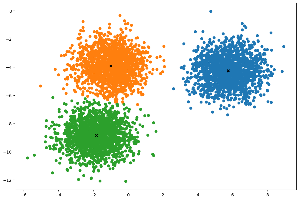

• However, optimized PyTorch version was a bit quicker than vectorized numpy implementation (.004 seconds vs .007 seconds).

Linear Regression

• Perform gradient descent using the following equations:
• dw = (1/N)*sum(2x(y_hat-y))
• db = (1/N)*sum(2(y_hat-y))
• w = w - lr*dw
• b = b - lr*db

class LinearRegression:
    def __init__(self, learning_rate=0.001, n_iters=1000):
        self.lr = learning_rate
        self.n_iters = n_iters
        self.weights = None
        self.bias = None

    def fit(self, X, y):
        self.n_examples, self.n_feats = X.shape
        self.weights = np.zeros(self.n_feats)
        self.bias = 0
        for i in range(self.n_iters):
           
            y_pred = X @ self.weights + self.bias
            if i == 0: print("X.shape, y_pred.shape: ", X.shape, y_pred.shape)

            dw = (2/self.n_examples)*np.dot(X.T,y_pred-y)
            db = (2/self.n_examples)*np.sum(y_pred-y) #np.dot(np.ones(self.n_examples),y_pred-y)
            if i == 0: print("dw.shape, db.shape: ", dw.shape, db.shape)


            self.weights -= self.lr*dw
            self.bias -= self.lr*db
        
    def predict(self, X):
        return X @ self.weights + self.bias

X, y = datasets.make_regression(
        n_samples=100, n_features=1, noise=20, random_state=4
    )

print(X.shape, y.shape)
X_train, X_test, y_train, y_test = train_test_split(
    X, y, test_size=0.2, random_state=1234
)
def mean_squared_error(y_test, predictions):
    return np.mean((y_test-predictions)**2)
def r2_score(y_test, predictions):
    ss_res = np.sum((y_test-predictions)**2) 
    ss_tot = np.sum((y_test-np.mean(y_test))**2) 
    return 1 - (ss_res/ss_tot)
regressor = LinearRegression(learning_rate=0.01, n_iters=1000)
regressor.fit(X_train, y_train)
predictions = regressor.predict(X_test)
print(predictions.shape)
print(predictions)
mse = mean_squared_error(y_test, predictions)
print("MSE:", mse)

accu = r2_score(y_test, predictions)
print("Accuracy:", accu)

y_pred_line = regressor.predict(X)
cmap = plt.get_cmap("viridis")
fig = plt.figure(figsize=(8, 6))
m1 = plt.scatter(X_train, y_train, color=cmap(0.9), s=10)
m2 = plt.scatter(X_test, y_test, color=cmap(0.5), s=10)
plt.plot(X, y_pred_line, color="black", linewidth=2, label="Prediction")
plt.show()

(100, 1) (100,)
X.shape, y_pred.shape:  (80, 1) (80,)
dw.shape, db.shape:  (1,) ()
(20,)
[  90.07911867   65.22240301  -45.69498186  -82.49167298   20.93910431
  -73.92513193  -14.90998903  151.65799643   14.01724561 -102.29561058
   15.56851863   41.60448602   26.20320259   38.12125411   37.38360674
  -37.35823254  -83.12683724   26.30425075   38.13183211   29.45312701]
MSE: 305.7741316085243
Accuracy: 0.9247515208337563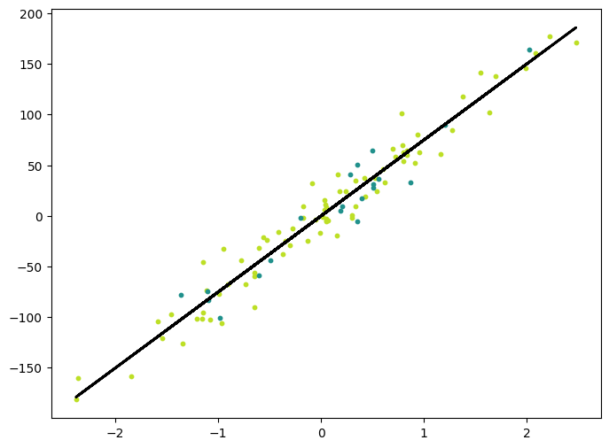

class LinearRegressionTorch:
    """Can use torch.autograd automatic differentiation for gradient updates"""
    def __init__(self, learning_rate=0.001, n_iters=1000):
        self.lr = learning_rate
        self.n_iters = n_iters
        self.weights = None
        self.bias = None

    def fit(self, X, y):
        self.n_examples, self.n_feats = X.shape
        self.weights = torch.zeros(self.n_feats, requires_grad=True)#, torch.dtype='torch.float32')
        self.bias = torch.zeros(1,requires_grad=True)
        optimizer = torch.optim.SGD([self.weights, self.bias], lr=self.lr)
        
        for _ in range(self.n_iters):
            y_pred = X @ self.weights + self.bias
            loss = torch.mean((y_pred-y)**2)
            loss.backward()
            optimizer.step()
            optimizer.zero_grad()


    def predict(self, X):
        with torch.no_grad():
            return X @ self.weights + self.bias

X, y = datasets.make_regression(
        n_samples=100, n_features=1, noise=20, random_state=4
    )
X, y = torch.tensor(X,  dtype=torch.float32), torch.tensor(y,  dtype=torch.float32)
print(X.shape, y.shape)
X_train, X_test, y_train, y_test = train_test_split(
    X, y, test_size=0.2, random_state=1234
)
def mean_squared_error(y_test, predictions):
    return torch.mean((y_test-predictions)**2)
def r2_score(y_test, predictions):
    ss_res = torch.sum((y_test-predictions)**2) 
    ss_tot = torch.sum((y_test-torch.mean(y_test))**2) 
    return 1 - (ss_res/ss_tot)
regressor = LinearRegressionTorch(learning_rate=0.01, n_iters=1000)
regressor.fit(X_train, y_train)
predictions = regressor.predict(X_test)
print(predictions.shape)
print(predictions)
mse = mean_squared_error(y_test, predictions)
print("MSE:", mse)

accu = r2_score(y_test, predictions)
print("Accuracy:", accu)

y_pred_line = regressor.predict(X).detach().numpy()
cmap = plt.get_cmap("viridis")
fig = plt.figure(figsize=(8, 6))
m1 = plt.scatter(X_train.detach().numpy(), y_train.detach().numpy(), color=cmap(0.9), s=10)
m2 = plt.scatter(X_test.detach().numpy(), y_test.detach().numpy(), color=cmap(0.5), s=10)
plt.plot(X.detach().numpy(), y_pred_line, color="black", linewidth=2, label="Prediction")
plt.show()

torch.Size([100, 1]) torch.Size([100])
torch.Size([20])
tensor([  90.0789,   65.2223,  -45.6949,  -82.4915,   20.9391,  -73.9249,
         -14.9099,  151.6576,   14.0172, -102.2954,   15.5685,   41.6044,
          26.2031,   38.1212,   37.3835,  -37.3581,  -83.1266,   26.3042,
          38.1317,   29.4531])
MSE: tensor(305.7739)
Accuracy: tensor(0.9248)

import torch.nn as nn
class LinearRegressionIdiomaticTorch(nn.Module):
    """Can use torch.autograd automatic differentiation for gradient updates"""
    def __init__(self, input_dim, output_dim=1):
        super().__init__()
        self.linear = nn.Linear(input_dim,output_dim)

    def forward(self, X):
        return self.linear(X)
    

X, y = datasets.make_regression(
        n_samples=100, n_features=1, noise=20, random_state=4
    )
X, y = torch.tensor(X,  dtype=torch.float32), torch.tensor(y,  dtype=torch.float32)#.view(-1,1)
print(X.shape, y.shape)
X_train, X_test, y_train, y_test = train_test_split(
    X, y, test_size=0.2, random_state=1234
)
model = LinearRegressionIdiomaticTorch(input_dim=X.shape[1])

# Training loop
n_iters = 1000
criterion = nn.MSELoss()
optimizer = torch.optim.SGD(model.parameters(), lr = 0.1)
for i in range(n_iters):
    optimizer.zero_grad()
    y_pred = model(X_train)
    if i==0: print('Shapes: y_pred.shape,y_train.shape', y_pred.shape,y_train.shape)
    loss = criterion(y_pred.view(-1),y_train) # .view(-1) CRITICAL!
    loss.backward()
    optimizer.step()


with torch.no_grad():
    predictions = model(X_test)
    # print("predictions: ")
    # print(predictions)

mse = mean_squared_error(y_test, predictions)
print("MSE:", mse)

accu = r2_score(y_test, predictions)
print("Accuracy:", accu)
with torch.no_grad():
    y_pred_line = model(X).detach().numpy()
cmap = plt.get_cmap("viridis")
fig = plt.figure(figsize=(8, 6))
m1 = plt.scatter(X_train.detach().numpy(), y_train.detach().numpy(), color=cmap(0.9), s=10)
m2 = plt.scatter(X_test.detach().numpy(), y_test.detach().numpy(), color=cmap(0.5), s=10)
plt.plot(X.detach().numpy(), y_pred_line, color="black", linewidth=2, label="Prediction")
plt.show()

torch.Size([100, 1]) torch.Size([100])
Shapes: y_pred.shape,y_train.shape torch.Size([80, 1]) torch.Size([80])
MSE: 305.7741
Accuracy: 0.924751527892842

• Learning moment (post conversing with GPT-40 Mini):

  While broadcasting allows the calculations to work, the gradients can behave differently based on how the operations are laid out, especially for loss functions that rely on precise error metrics across dimensions. When you switch to using shapes of (80,) explicitly, you simplify the relationship, making it easier for the backpropagation process to understand and compute the gradients correctly.

  Thus, while the shapes may become mathematically compatible, the implicit behavior of broadcasting and element-wise operations fundamentally leads to differing gradient flows. Clarity in tensor shapes is incredibly important for ensuring that operations function as anticipated in deep learning frameworks like PyTorch.

• I had loss = criterion(y_pred.view(-1),y_train) without the .view(-1) at first, which led to just the intercept being estimated! (got a horizontal line as prediction). It seems that there’s are intricacies with broadcasting in loss calculations. It’s best to explicitly convert tensors to the right shape so that PyTorch computes the gradients correctly.

import torch.nn as nn
class SimpleNN(nn.Module):
    """Can use torch.autograd automatic differentiation for gradient updates"""
    def __init__(self, input_dim, output_dim=1,hidden_dim =10):
        super().__init__()
        self.ln1 = nn.Linear(input_dim,hidden_dim)
        self.relu = nn.ReLU()
        self.ln2 = nn.Linear(hidden_dim,output_dim)

    def forward(self, X):
        x = self.ln1(X)
        x = self.ln2(self.relu(x))
        return x

model = SimpleNN(input_dim=X.shape[1])

# Training loop
n_iters = 1000
criterion = nn.MSELoss()
optimizer = torch.optim.SGD(model.parameters(), lr = 0.01)
for _ in range(n_iters):
    y_pred = model(X_train)
    loss = criterion(y_pred.view(-1),y_train)
    loss.backward()
    optimizer.step()
    optimizer.zero_grad()


with torch.no_grad():
    predictions = model(X_test)
   # print(predictions)

mse = mean_squared_error(y_test, predictions)
print("MSE:", mse)

accu = r2_score(y_test, predictions)
print("Accuracy:", accu)
with torch.no_grad():
    y_pred_line = model(X).detach().numpy()
cmap = plt.get_cmap("viridis")
fig = plt.figure(figsize=(8, 6))
m1 = plt.scatter(X_train.detach().numpy(), y_train.detach().numpy(), color=cmap(0.9), s=10)
m2 = plt.scatter(X_test.detach().numpy(), y_test.detach().numpy(), color=cmap(0.5), s=10)


plt.plot(X.detach().numpy(), y_pred_line, color="black", linewidth=1, label="Prediction")
plt.show()

MSE: 341.73175
Accuracy: 0.9159026386036382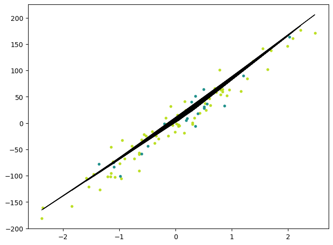

Logistic Regression

• Gradient updates are same as in linear regression, but since the targets are 0/1, convert predictions to probabilities via sigmoid.

class LogisticRegression:
    def __init__(self, learning_rate=0.001, n_iters=1000):
        self.lr = learning_rate
        self.n_iters = n_iters
        self.weights = None
        self.bias = None

    def fit(self, X, y):
       self.n_examples, self.n_feats = X.shape
       self.weights = np.zeros(self.n_feats)
       self.bias = 0
       for _ in range(self.n_iters):
           y_pred = self._sigmoid(X@self.weights+self.bias)

           dw = (2/self.n_examples)*np.dot(X.T,y_pred-y)
           db = (2/self.n_examples)*np.sum(y_pred-y)

           self.weights -= self.lr * dw
           self.bias -= self.lr * db

    def predict(self, X):
        probs = self._sigmoid(X@self.weights+self.bias)
        return np.array([1 if prob > 0.5 else 0 for prob in probs ])

    def _sigmoid(self, x):
        return 1/(1+np.exp(-x))


# Testing
if __name__ == "__main__":
    # Imports
    from sklearn.model_selection import train_test_split
    from sklearn import datasets

    def accuracy(y_true, y_pred):
        accuracy = np.sum(y_true == y_pred) / len(y_true)
        return accuracy

    bc = datasets.load_breast_cancer()
    X, y = bc.data, bc.target
    X_train, X_test, y_train, y_test = train_test_split(
        X, y, test_size=0.2, random_state=1234
    )

    regressor = LogisticRegression(learning_rate=0.00005, n_iters=1000) # think they forgot 2x in grad updates, halving lr to get same accuracy
    regressor.fit(X_train, y_train)
    predictions = regressor.predict(X_test)

    print("LR classification accuracy:", accuracy(y_test, predictions))

LR classification accuracy: 0.9298245614035088

• PyTorch version is not very numerically stable, increased precision to torch.float64 to match that of numpy, experimented with different random seeds until found one of the better ones. BCEWithLogitsLoss may help the issue in the future. Either way, there seems to be a about 3 different ‘valleys’ where the algorithm ends up ‘converging’, likely local minima on the loss surface.

class LogisticRegressionTorch(nn.Module):
    def __init__(self, input_dims):
        super().__init__()
        self.ff = nn.Linear(input_dims,1,dtype=torch.float64)
        self.sigm = nn.Sigmoid()

    def forward(self, X):
       return self.sigm(self.ff(X))


# Imports
from sklearn.model_selection import train_test_split
from sklearn import datasets


bc = datasets.load_breast_cancer()
X, y = torch.tensor(bc.data,dtype = torch.float64), torch.tensor(bc.target, dtype = torch.float64).view(-1,1)

X_train, X_test, y_train, y_test = train_test_split(
    X, y, test_size=0.2, random_state=1234
)
torch.manual_seed(7777777) # a bit unstable, depending on random seed, this is one of the better ones
n_iters, lr = 10000, .00005
n_examples, n_feats = X.shape
log_reg = LogisticRegressionTorch(n_feats)
loss_fn = nn.BCELoss() # may consider nn.BCEWithLogitsLoss() for numeric stability
optimizer = torch.optim.SGD(log_reg.parameters(),lr)
for _ in range(n_iters):
    optimizer.zero_grad()
    y_pred = log_reg(X_train).view(-1,1)
    loss = loss_fn(y_pred,y_train)
    loss.backward()
    optimizer.step()

with torch.no_grad():
    y_pred_test = log_reg(X_test)
    y_pred_test_class = y_pred_test.round()
    print(list(zip(y_pred_test_class,y_test)))

correct = (y_pred_test_class==y_test).float()
accuracy = correct.sum()/len(correct)
print("LR classification accuracy:", accuracy.item())

[(tensor([1.], dtype=torch.float64), tensor([1.], dtype=torch.float64)), (tensor([1.], dtype=torch.float64), tensor([1.], dtype=torch.float64)), (tensor([1.], dtype=torch.float64), tensor([1.], dtype=torch.float64)), (tensor([1.], dtype=torch.float64), tensor([1.], dtype=torch.float64)), (tensor([1.], dtype=torch.float64), tensor([1.], dtype=torch.float64)), (tensor([1.], dtype=torch.float64), tensor([1.], dtype=torch.float64)), (tensor([0.], dtype=torch.float64), tensor([0.], dtype=torch.float64)), (tensor([1.], dtype=torch.float64), tensor([1.], dtype=torch.float64)), (tensor([0.], dtype=torch.float64), tensor([0.], dtype=torch.float64)), (tensor([0.], dtype=torch.float64), tensor([0.], dtype=torch.float64)), (tensor([0.], dtype=torch.float64), tensor([0.], dtype=torch.float64)), (tensor([1.], dtype=torch.float64), tensor([1.], dtype=torch.float64)), (tensor([1.], dtype=torch.float64), tensor([1.], dtype=torch.float64)), (tensor([1.], dtype=torch.float64), tensor([1.], dtype=torch.float64)), (tensor([1.], dtype=torch.float64), tensor([1.], dtype=torch.float64)), (tensor([0.], dtype=torch.float64), tensor([0.], dtype=torch.float64)), (tensor([1.], dtype=torch.float64), tensor([1.], dtype=torch.float64)), (tensor([1.], dtype=torch.float64), tensor([1.], dtype=torch.float64)), (tensor([1.], dtype=torch.float64), tensor([1.], dtype=torch.float64)), (tensor([0.], dtype=torch.float64), tensor([0.], dtype=torch.float64)), (tensor([1.], dtype=torch.float64), tensor([1.], dtype=torch.float64)), (tensor([0.], dtype=torch.float64), tensor([0.], dtype=torch.float64)), (tensor([0.], dtype=torch.float64), tensor([0.], dtype=torch.float64)), (tensor([0.], dtype=torch.float64), tensor([0.], dtype=torch.float64)), (tensor([0.], dtype=torch.float64), tensor([0.], dtype=torch.float64)), (tensor([0.], dtype=torch.float64), tensor([1.], dtype=torch.float64)), (tensor([0.], dtype=torch.float64), tensor([0.], dtype=torch.float64)), (tensor([1.], dtype=torch.float64), tensor([1.], dtype=torch.float64)), (tensor([1.], dtype=torch.float64), tensor([1.], dtype=torch.float64)), (tensor([1.], dtype=torch.float64), tensor([1.], dtype=torch.float64)), (tensor([1.], dtype=torch.float64), tensor([1.], dtype=torch.float64)), (tensor([1.], dtype=torch.float64), tensor([1.], dtype=torch.float64)), (tensor([0.], dtype=torch.float64), tensor([0.], dtype=torch.float64)), (tensor([1.], dtype=torch.float64), tensor([1.], dtype=torch.float64)), (tensor([1.], dtype=torch.float64), tensor([1.], dtype=torch.float64)), (tensor([1.], dtype=torch.float64), tensor([1.], dtype=torch.float64)), (tensor([1.], dtype=torch.float64), tensor([1.], dtype=torch.float64)), (tensor([0.], dtype=torch.float64), tensor([0.], dtype=torch.float64)), (tensor([0.], dtype=torch.float64), tensor([0.], dtype=torch.float64)), (tensor([1.], dtype=torch.float64), tensor([1.], dtype=torch.float64)), (tensor([0.], dtype=torch.float64), tensor([0.], dtype=torch.float64)), (tensor([1.], dtype=torch.float64), tensor([1.], dtype=torch.float64)), (tensor([0.], dtype=torch.float64), tensor([0.], dtype=torch.float64)), (tensor([1.], dtype=torch.float64), tensor([1.], dtype=torch.float64)), (tensor([1.], dtype=torch.float64), tensor([1.], dtype=torch.float64)), (tensor([1.], dtype=torch.float64), tensor([1.], dtype=torch.float64)), (tensor([1.], dtype=torch.float64), tensor([1.], dtype=torch.float64)), (tensor([0.], dtype=torch.float64), tensor([0.], dtype=torch.float64)), (tensor([0.], dtype=torch.float64), tensor([0.], dtype=torch.float64)), (tensor([1.], dtype=torch.float64), tensor([1.], dtype=torch.float64)), (tensor([1.], dtype=torch.float64), tensor([1.], dtype=torch.float64)), (tensor([1.], dtype=torch.float64), tensor([1.], dtype=torch.float64)), (tensor([1.], dtype=torch.float64), tensor([1.], dtype=torch.float64)), (tensor([0.], dtype=torch.float64), tensor([0.], dtype=torch.float64)), (tensor([0.], dtype=torch.float64), tensor([0.], dtype=torch.float64)), (tensor([1.], dtype=torch.float64), tensor([1.], dtype=torch.float64)), (tensor([1.], dtype=torch.float64), tensor([1.], dtype=torch.float64)), (tensor([1.], dtype=torch.float64), tensor([1.], dtype=torch.float64)), (tensor([1.], dtype=torch.float64), tensor([1.], dtype=torch.float64)), (tensor([0.], dtype=torch.float64), tensor([0.], dtype=torch.float64)), (tensor([1.], dtype=torch.float64), tensor([1.], dtype=torch.float64)), (tensor([1.], dtype=torch.float64), tensor([1.], dtype=torch.float64)), (tensor([1.], dtype=torch.float64), tensor([1.], dtype=torch.float64)), (tensor([1.], dtype=torch.float64), tensor([1.], dtype=torch.float64)), (tensor([1.], dtype=torch.float64), tensor([1.], dtype=torch.float64)), (tensor([0.], dtype=torch.float64), tensor([0.], dtype=torch.float64)), (tensor([0.], dtype=torch.float64), tensor([0.], dtype=torch.float64)), (tensor([1.], dtype=torch.float64), tensor([1.], dtype=torch.float64)), (tensor([1.], dtype=torch.float64), tensor([1.], dtype=torch.float64)), (tensor([0.], dtype=torch.float64), tensor([0.], dtype=torch.float64)), (tensor([1.], dtype=torch.float64), tensor([1.], dtype=torch.float64)), (tensor([0.], dtype=torch.float64), tensor([0.], dtype=torch.float64)), (tensor([1.], dtype=torch.float64), tensor([1.], dtype=torch.float64)), (tensor([1.], dtype=torch.float64), tensor([0.], dtype=torch.float64)), (tensor([1.], dtype=torch.float64), tensor([1.], dtype=torch.float64)), (tensor([1.], dtype=torch.float64), tensor([1.], dtype=torch.float64)), (tensor([1.], dtype=torch.float64), tensor([1.], dtype=torch.float64)), (tensor([0.], dtype=torch.float64), tensor([0.], dtype=torch.float64)), (tensor([1.], dtype=torch.float64), tensor([1.], dtype=torch.float64)), (tensor([0.], dtype=torch.float64), tensor([0.], dtype=torch.float64)), (tensor([1.], dtype=torch.float64), tensor([1.], dtype=torch.float64)), (tensor([1.], dtype=torch.float64), tensor([1.], dtype=torch.float64)), (tensor([1.], dtype=torch.float64), tensor([1.], dtype=torch.float64)), (tensor([1.], dtype=torch.float64), tensor([0.], dtype=torch.float64)), (tensor([0.], dtype=torch.float64), tensor([0.], dtype=torch.float64)), (tensor([0.], dtype=torch.float64), tensor([0.], dtype=torch.float64)), (tensor([0.], dtype=torch.float64), tensor([0.], dtype=torch.float64)), (tensor([0.], dtype=torch.float64), tensor([0.], dtype=torch.float64)), (tensor([0.], dtype=torch.float64), tensor([1.], dtype=torch.float64)), (tensor([1.], dtype=torch.float64), tensor([0.], dtype=torch.float64)), (tensor([1.], dtype=torch.float64), tensor([1.], dtype=torch.float64)), (tensor([1.], dtype=torch.float64), tensor([0.], dtype=torch.float64)), (tensor([1.], dtype=torch.float64), tensor([1.], dtype=torch.float64)), (tensor([0.], dtype=torch.float64), tensor([0.], dtype=torch.float64)), (tensor([1.], dtype=torch.float64), tensor([0.], dtype=torch.float64)), (tensor([1.], dtype=torch.float64), tensor([1.], dtype=torch.float64)), (tensor([1.], dtype=torch.float64), tensor([1.], dtype=torch.float64)), (tensor([1.], dtype=torch.float64), tensor([1.], dtype=torch.float64)), (tensor([1.], dtype=torch.float64), tensor([1.], dtype=torch.float64)), (tensor([1.], dtype=torch.float64), tensor([1.], dtype=torch.float64)), (tensor([0.], dtype=torch.float64), tensor([0.], dtype=torch.float64)), (tensor([0.], dtype=torch.float64), tensor([0.], dtype=torch.float64)), (tensor([1.], dtype=torch.float64), tensor([1.], dtype=torch.float64)), (tensor([1.], dtype=torch.float64), tensor([1.], dtype=torch.float64)), (tensor([0.], dtype=torch.float64), tensor([0.], dtype=torch.float64)), (tensor([1.], dtype=torch.float64), tensor([1.], dtype=torch.float64)), (tensor([1.], dtype=torch.float64), tensor([1.], dtype=torch.float64)), (tensor([0.], dtype=torch.float64), tensor([0.], dtype=torch.float64)), (tensor([0.], dtype=torch.float64), tensor([0.], dtype=torch.float64)), (tensor([1.], dtype=torch.float64), tensor([1.], dtype=torch.float64)), (tensor([0.], dtype=torch.float64), tensor([0.], dtype=torch.float64)), (tensor([0.], dtype=torch.float64), tensor([1.], dtype=torch.float64)), (tensor([0.], dtype=torch.float64), tensor([0.], dtype=torch.float64)), (tensor([0.], dtype=torch.float64), tensor([0.], dtype=torch.float64))]
LR classification accuracy: 0.9298245906829834

PCA

• Subtract the mean from X
• Calculate Cov(X,X)
• Calculate eigenvectors and eigenvalues of the covariance matrix
• Sort the eigenvectors according to their eigenvalues in decreasing order
• Choose the first k eigenvectors as the new k dimensions
• Transform the original n-dimensional data points into k dimensions by projecting with dot product

Some explanation for why this works from GPT 4omini, found points 3 and 4 to be particularly useful:

In PCA, we start with a dataset represented as a matrix, and we want to identify the directions (principal components) in which the data varies the most. Here’s how eigenvectors and eigenvalues come into play:

1. Covariance Matrix: The covariance matrix of the dataset captures how the variables vary with respect to each other. When you compute the covariance matrix, you’re essentially summarizing the relationships and variances of the dimensions.

2. Eigenvalues and Eigenvectors: When you find the eigenvalues and eigenvectors of the covariance matrix, the eigenvectors represent the directions of maximum variance (principal components), and the corresponding eigenvalues quantify the amount of variance in those directions. Specifically:

   • An eigenvector with a larger eigenvalue indicates that there is more variance in the data along that direction.
   • Conversely, a smaller eigenvalue indicates less variance.

3. Preservation of Variance: The reason the eigenvectors corresponding to the largest eigenvalues preserve the most variance is that they effectively align with the directions where the data is most spread out. When you project the data onto these eigenvectors (principal components), you are capturing the largest portion of the data’s variability.

4. Transformation and Basis: Regarding your mention of transforming the standard basis, think of it this way: The largest eigenvalues indicate how much “stretching” occurs along the directions defined by their corresponding eigenvectors. These are the directions where the data points are furthest apart from each other, hence preserving the variance best. The eigenvalues tell you how much variance is retained when the data is projected onto the eigenvectors.

In summary, in PCA, the eigenvectors of the covariance matrix with the largest eigenvalues indicate the directions of maximum variance, and projecting data onto these eigenvectors retains the most significant patterns and variability from the original dataset. This is why they are so crucial for dimensionality reduction while retaining important information.

class PCA:
    def __init__(self, n_components):
        self.n_components = n_components
        self.components = None
        self.mean = None

    def fit(self, X, debug = False):
        self.X_bar = np.mean(X,axis=0) # store so as to be able to subtract it later in transform
        X-= self.X_bar  #subtract teh mean from X
        cov = X.T @ X #calculate cov of X
        eigenvalues, eigenvectors = np.linalg.eig(cov) #calculate eigenvectors/eigenvalues
        if debug: print("eigenvalues, eigenvectors ", eigenvalues, eigenvectors)
        eigenvectors = eigenvectors[np.argsort(eigenvalues)[::-1]] # Sort the eigenvectors according to their eigenvalues in decreasing order
        if debug: print(eigenvectors) 
        self.components = eigenvectors[:self.n_components] # Choose the first k eigenvectors as the new k dimensions
        if debug: print(self.components) 
           

    def transform(self, X):
        X -= self.X_bar # Must subtract the mean to center new data consistently!
        # Transform the original n-dimensional data points into k dimensions by projecting with dot product 
        return X @ self.components.T     
       
# Testing
if __name__ == "__main__":
    # Imports
    import matplotlib.pyplot as plt
    from sklearn import datasets

    # data = datasets.load_digits()
    data = datasets.load_iris()
    X = data.data
    y = data.target

    # Project the data onto the 2 primary principal components
    pca = PCA(2)
    pca.fit(X,debug = True)
    X_projected = pca.transform(X)

    print("Shape of X:", X.shape)
    print("Shape of transformed X:", X_projected.shape)

    x1 = X_projected[:, 0]
    x2 = X_projected[:, 1]

    plt.scatter(
        x1, x2, c=y, edgecolor="none", alpha=0.8, cmap=plt.cm.get_cmap("viridis", 3)
    )

    plt.xlabel("Principal Component 1")
    plt.ylabel("Principal Component 2")
    plt.colorbar()
    plt.show()

eigenvalues, eigenvectors  [630.0080142   36.15794144  11.65321551   3.55142885] [[ 0.36138659 -0.65658877 -0.58202985  0.31548719]
 [-0.08452251 -0.73016143  0.59791083 -0.3197231 ]
 [ 0.85667061  0.17337266  0.07623608 -0.47983899]
 [ 0.3582892   0.07548102  0.54583143  0.75365743]]
[[ 0.36138659 -0.65658877 -0.58202985  0.31548719]
 [-0.08452251 -0.73016143  0.59791083 -0.3197231 ]
 [ 0.85667061  0.17337266  0.07623608 -0.47983899]
 [ 0.3582892   0.07548102  0.54583143  0.75365743]]
[[ 0.36138659 -0.65658877 -0.58202985  0.31548719]
 [-0.08452251 -0.73016143  0.59791083 -0.3197231 ]]
Shape of X: (150, 4)
Shape of transformed X: (150, 2)

/tmp/ipykernel_6079/3178312349.py:47: MatplotlibDeprecationWarning: The get_cmap function was deprecated in Matplotlib 3.7 and will be removed in 3.11. Use ``matplotlib.colormaps[name]`` or ``matplotlib.colormaps.get_cmap()`` or ``pyplot.get_cmap()`` instead.
  x1, x2, c=y, edgecolor="none", alpha=0.8, cmap=plt.cm.get_cmap("viridis", 3)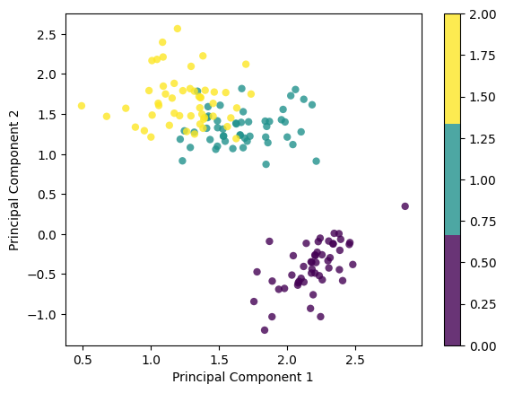

class PCATorch:
    def __init__(self, n_components):
        self.n_components = n_components
        self.components = None
        self.mean = None

    def fit(self, X, debug = False):
        self.X_bar = torch.mean(X,axis=0) # store so as to be able to subtract it later in transform
        X-= self.X_bar  #subtract teh mean from X
        cov = X.T @ X #calculate cov of X
        eigenvalues_complex, eigenvectors_complex = torch.linalg.eig(cov) #calculate eigenvectors/eigenvalues; return complex
        eigenvalues, eigenvalues_imag = eigenvalues_complex.real, eigenvalues_complex.imag
        eigenvectors, eigenvectors_imag = eigenvectors_complex.real, eigenvectors_complex.imag
        assert torch.allclose(eigenvalues_imag, torch.zeros_like(eigenvalues_imag),atol=1e-6), "Imaginary parts of eigenvalues are not zero"
        assert torch.allclose(eigenvectors_imag, torch.zeros_like(eigenvectors_imag),atol=1e-6), "Imaginary parts of eigenvectors are not zero"
        if debug: print("eigenvalues, eigenvectors ", eigenvalues, eigenvectors)
        eigenvectors = eigenvectors[torch.argsort(eigenvalues,descending=True)] # Sort the eigenvectors according to their eigenvalues in decreasing order
        if debug: print(eigenvectors) 
        self.components = eigenvectors[:self.n_components] # Choose the first k eigenvectors as the new k dimensions
        if debug: print(self.components) 
           

    def transform(self, X):
        X -= self.X_bar # Must subtract the mean to center new data consistently!
        # Transform the original n-dimensional data points into k dimensions by projecting with dot product 
        return X @ self.components.T     
       
# Testing
if __name__ == "__main__":
    # Imports
    import matplotlib.pyplot as plt
    from sklearn import datasets

    # data = datasets.load_digits()
    data = datasets.load_iris()
    X = torch.tensor(data.data,dtype = torch.float32)
    y = torch.tensor(data.target, dtype=torch.float32)

    # Project the data onto the 2 primary principal components
    pca = PCATorch(2)
    pca.fit(X,debug = True)
    X_projected = pca.transform(X)

    print("Shape of X:", X.shape)
    print("Shape of transformed X:", X_projected.shape)

    x1 = X_projected[:, 0]
    x2 = X_projected[:, 1]

    plt.scatter(
        x1, x2, c=y, edgecolor="none", alpha=0.8, cmap=plt.cm.get_cmap("viridis", 3)
    )

    plt.xlabel("Principal Component 1")
    plt.ylabel("Principal Component 2")
    plt.colorbar()
    plt.show()

eigenvalues, eigenvectors  tensor([630.0081,  36.1579,  11.6532,   3.5514]) tensor([[-0.3614, -0.6566, -0.5820,  0.3155],
        [ 0.0845, -0.7302,  0.5979, -0.3197],
        [-0.8567,  0.1734,  0.0762, -0.4798],
        [-0.3583,  0.0755,  0.5458,  0.7537]])
tensor([[-0.3614, -0.6566, -0.5820,  0.3155],
        [ 0.0845, -0.7302,  0.5979, -0.3197],
        [-0.8567,  0.1734,  0.0762, -0.4798],
        [-0.3583,  0.0755,  0.5458,  0.7537]])
tensor([[-0.3614, -0.6566, -0.5820,  0.3155],
        [ 0.0845, -0.7302,  0.5979, -0.3197]])
Shape of X: torch.Size([150, 4])
Shape of transformed X: torch.Size([150, 2])

/tmp/ipykernel_6079/1788467269.py:51: MatplotlibDeprecationWarning: The get_cmap function was deprecated in Matplotlib 3.7 and will be removed in 3.11. Use ``matplotlib.colormaps[name]`` or ``matplotlib.colormaps.get_cmap()`` or ``pyplot.get_cmap()`` instead.
  x1, x2, c=y, edgecolor="none", alpha=0.8, cmap=plt.cm.get_cmap("viridis", 3)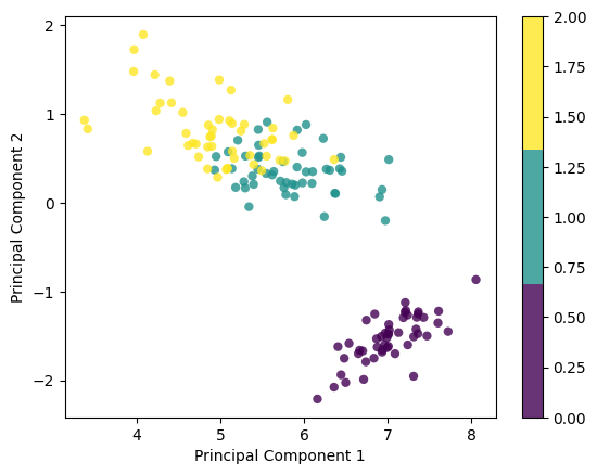

Decision Tree

• Training:

  • Calculate information gain (IG) with each possible split. IG = Entropy(parent) - weighted avg of Entropy(children). Entropy = - Sum(p(X)*log(p(X))), where p(X)=(#x/n)
  • Divide set with that feature and value that gives the greatest IG
  • Divide tree and do the same for all created branches
  • … repeat until reach stopping criteria (max depth, min # samples, min impurity decrease).

• Testing:

  • Follow the tree until you reach a leaf node
  • Return the most common class label

• Not implementing this in PyTorch since it’s a mostly iterative algorithm and don’t expect a gain from GPU parallelization.

• Code overview:

  • Make a Node class (along with feature, threshold, left, right, value properties) along including a is_leaf_node helper identifying nodes with a value as leaf nodes.
  • Make a DecisionTree class containing min_samples_split, max_depth, n_feats, and root properties, as well as the rest of the functionality.
    • The fit method would just make sure self.n_feats is set correctly by not exceeding self.n_feats passed at initialization and call the *_fit* recursive helper.
    • The *_fit* method
      • Gets n_labels via len(np.unique(y)) from y, n_samples, n_feats from X.shape.
      • Gets the leaf_value via collections.Counter to use for base case of returning Node(value=leaf_value) if depth or min samples split conditions are met (or there’s just one label).
        
      • Finds indices of features to split on via np.random.choice and calls *_best_criteria* method, which iteratively finds max gain along with best_feat_idx, best_thresh by looping through indices and thresholds via np.unique(X_col). It uses *_information_gain* and entropy helpers (see below) for finding the max gain.
      • best_feat_idx and best_thresh are used to *_split* X at best_feat_idx based on best_thresh. The *_split* method simply calls np.argwhere to find the left_idxs and right_idxs.
      • Then left = self._fit(X[left_idxs, :], y[left_idxs], depth + 1), and right is defined similarly. Return Node(feature=best_feat_idx, threshold=best_thresh, left=left, right=right)
      • Information Gain is Entropy(parent) - weighted avg of Entropy(children). Use *_split* to get left_idxs and right_idxs along with a simple weighted average calculations, just make sure to return 0 if left_idxs or right_idxs are empty.
        
      • Entropy = - Sum(p(Y)*log(p(Y))), where p(Y)=(#y/n) can be computed via np.bincount(y)
    • The predict method calls *_traverse_tree* for each example x in X, starting traversal at the root.
      • *_traverse_tree* is recursive, traversing at node.left if x[node.feature] <= node.threshold, similarly for right. Keep example x the same, of course, since traverse from root to leaf node for each example. Base case is node.leaf_node(), in which case return node.value.

class Node:
    def __init__(self, feature=None, threshold=None, left=None, right=None, *, value=None):
        """
        Initialize a node in the decision tree.
        """
        self.feature = feature
        self.threshold = threshold
        self.left = left
        self.right = right
        self.value = value

    def is_leaf_node(self):
        """
        Check if the node is a leaf node.
        """
        return self.value is not None

class DecisionTree:
    def __init__(self, min_samples_split=2, max_depth=100, n_feats=None):
        """
        Initialize the decision tree.
        """
        self.min_samples_split = min_samples_split
        self.max_depth = max_depth
        self.n_feats = n_feats
        self.root = None

    def fit(self, X, y):
        """
        Fit the decision tree to the data by calling the _fit helper.
        """
        self.n_feats = X.shape[1] if not self.n_feats else min(X.shape[1], self.n_feats)
        self.root = self._fit(X, y)

    def _fit(self, X, y, depth=0):
        """
        Recursively grow the decision tree using _best_criteria and _split helpers. 
        """
        n_labels = len(np.unique(y))
        n_samples, n_feats = X.shape
        
        # Check stopping criteria
        leaf_value = collections.Counter(y).most_common(1)[0][0]
        if depth >= self.max_depth or n_samples < self.min_samples_split or n_labels == 1:
            return Node(value=leaf_value)

        # Find the best split
        feat_idxs = np.random.choice(n_feats, size=self.n_feats, replace=False)
        best_feat_idx, best_thresh = self._best_criteria(X, y, feat_idxs)

        # Create child nodes recursively
        left_idxs, right_idxs = self._split(X[:, best_feat_idx], best_thresh)
        left = self._fit(X[left_idxs, :], y[left_idxs], depth + 1)
        right = self._fit(X[right_idxs, :], y[right_idxs], depth + 1)
        return Node(feature=best_feat_idx, threshold=best_thresh, left=left, right=right)

    def _best_criteria(self, X, y, feat_idxs):
        """
        Find the best split criteria.
        """
        max_gain = -float('inf')
        best_feat_idx, best_thresh = None, None
        for feat_idx in feat_idxs:
            X_col = X[:, feat_idx]
            thresholds = np.unique(X_col)
            for thresh in thresholds:
                gain = self._information_gain(y, X_col, thresh)
                if gain > max_gain:
                    max_gain, best_feat_idx, best_thresh = gain, feat_idx, thresh
        return best_feat_idx, best_thresh
    
    def _split(self, X_column, split_thresh):
        """
        Split the data based on the split threshold.
        """
        left_idxs = np.argwhere(X_column <= split_thresh).flatten()
        right_idxs = np.argwhere(X_column > split_thresh).flatten()
        return left_idxs, right_idxs

    @staticmethod
    def entropy(y):
        """
        Calculate the entropy of a label array.
        """
        hist = np.bincount(y)
        ps = hist / len(y)
        return -np.sum([p * np.log2(p) for p in ps if p > 0])

    def _information_gain(self, y, X_column, split_thresh):
        """
        Calculate the information gain of a split.
        """
        parent_entropy = DecisionTree.entropy(y)
        left_idxs, right_idxs = self._split(X_column, split_thresh)
        if len(left_idxs) == 0 or len(right_idxs) == 0:
            return 0

        n = len(y)
        n_left, n_right = len(left_idxs), len(right_idxs)
        e_left, e_right = DecisionTree.entropy(y[left_idxs]), DecisionTree.entropy(y[right_idxs])
        children_entropy = (n_left * e_left + n_right * e_right) / n
        return parent_entropy - children_entropy

    def predict(self, X):
        """
        Predict the class labels for the input data.
        """
        return np.array([self._traverse_tree(x, self.root) for x in X])

    def _traverse_tree(self, x, node):
        """
        Traverse the tree to make a prediction.
        """
        if node.is_leaf_node():
            return node.value
        if x[node.feature] <= node.threshold:
            return self._traverse_tree(x, node.left)
        else:
            return self._traverse_tree(x, node.right)

if __name__ == "__main__":
    # Imports
    from sklearn import datasets
    from sklearn.model_selection import train_test_split

    def accuracy(y_true, y_pred):
        """
        Calculate the accuracy of predictions.
        """
        return np.sum(y_true == y_pred) / len(y_true)

    # Load dataset
    data = datasets.load_breast_cancer()
    X, y = data.data, data.target

    # Split dataset into training and testing sets
    X_train, X_test, y_train, y_test = train_test_split(X, y, test_size=0.2, random_state=1234)

    # Initialize and train the decision tree
    clf = DecisionTree(max_depth=20)
    clf.fit(X_train, y_train)

    # Make predictions and calculate accuracy
    y_pred = clf.predict(X_test)
    acc = accuracy(y_test, y_pred)

    print("Accuracy:", acc)

Accuracy: 0.9298245614035088

Random Forest

• Deviating from mlfromscratch/random_forest.py implementation by adding max_samples, which is customary in standard random forest implementations such as scikit’s. This allows the forest to get a greater sample variety during bootstrapping by making the rows selection random, in addition to feature selection, which is random for each decision tree.
• fit method loops over self.n_trees, taking a random sample of rows via np.random.choice, making X_sample and y_sample with it, constructing each DecisionTree, then fitting it on the samples. It appends each fitted tree to self.trees.
  
• predict method constructs an array of predictions from each individual tree predictions, swaps axes with np.swapaxes since we want all predictions for each sample to be grouped together, then returns array of most common labels for each pred (using the same logic as finding most common label for each decision tree).

class RandomForest:
    def __init__(self, n_trees=10, min_samples_split=2, max_samples = 10, max_depth=100, n_feats=None):
        self.n_trees = n_trees
        self.min_samples_split = min_samples_split
        self.max_samples = max_samples # add to be consistent with most implementations, including scikit's, choose total of max_samples from all samples for each tree
        self.max_depth = max_depth
        self.n_feats = n_feats
        self.trees = []

    def fit(self, X, y):
        self.trees = []
        for _ in range(self.n_trees):
            n_samples = X.shape[0]
            self.max_samples = min(X.shape[1], self.max_samples)
            bootstrap_examples_idxs = np.random.choice(n_samples, self.max_samples, replace=True) # bootstrap samples -> replace = True
            X_sample, y_sample = X[bootstrap_examples_idxs,:], y[bootstrap_examples_idxs] # unlike in tree, choosing ROWS/examples!  In tree, choose features.
            tree = DecisionTree(min_samples_split=self.min_samples_split, max_depth=self.max_depth, n_feats=self.n_feats)
            tree.fit(X_sample,y_sample)
            self.trees.append(tree)


    def predict(self, X):
        # will have [[x1_tree1_pred,x2_tree1_pred,x3_tree1_pred,...],[x1_tree2_pred,x2_tree2_pred,x3_tree2_pred,...],...]
        # want [[x1_tree1_pred,x1_tree2_pred,x1_tree3_pred,...],[x2_tree1_pred,x2_tree2_pred,x2_tree3_pred,...],...] -> np.swapaxes
        # In fit, each tree has been fit on the training data, now use tree's own fit method to make the prediction on new data.
        preds = np.array([tree.predict(X) for tree in self.trees])
        preds = np.swapaxes(preds,0,1)
        return np.array([self.most_common_label(pred) for pred in preds])

    def most_common_label(self,y):
        return collections.Counter(y).most_common(1)[0][0]


# Testing
if __name__ == "__main__":
    # Imports
    from sklearn import datasets
    from sklearn.model_selection import train_test_split

    def accuracy(y_true, y_pred):
        accuracy = np.sum(y_true == y_pred) / len(y_true)
        return accuracy

    data = datasets.load_breast_cancer()
    X = data.data
    y = data.target
    print(X.shape)
    X_train, X_test, y_train, y_test = train_test_split(
        X, y, test_size=0.2, random_state=1234
    )
    np.random.seed(117)
    clf = RandomForest(n_trees=5, max_depth=10, max_samples=25) #simple data, hard to surpass DecisionTree accuracy

    clf.fit(X_train, y_train)
    y_pred = clf.predict(X_test)
    acc = accuracy(y_test, y_pred)

    print("Accuracy:", acc)

(569, 30)
Accuracy: 0.9298245614035088

SVM

SVM Objective, source: https://www.youtube.com/watch?v=T9UcK-TxQGw

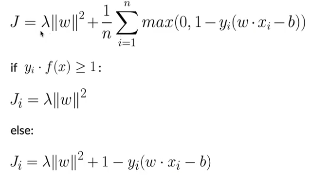
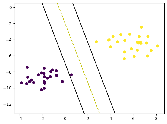
• Training:
  • Initialize the weights
  • Make sure y is in set([-1,1])
  • Apply grad update rules for n iterations
    • If y (wx-b)>=1, dw = 2 lambda w, db = 0
    • Else, dw = 2 lambda w - y x, db = y
• Prediction:
  • Calculate y = sign(wx-b)

import numpy as np


class SVM:
    def __init__(self, learning_rate=0.001, lambda_param=0.01, n_iters=1000):
        self.lr = learning_rate
        self.lambda_param = lambda_param
        self.n_iters = n_iters
        self.w = None
        self.b = None

    def fit(self, X, y):
        n_feats = X.shape[1]
        self.w, self.b = np.zeros(n_feats), 0
        y = np.where(y <=0, -1, 1)
        for _ in range(self.n_iters):
            for idx, x_i in enumerate(X):
                margin = y[idx]*(np.dot(x_i,self.w)-self.b)
                dw = np.where(margin>=1, 2*self.lambda_param*self.w, 2*self.lambda_param*self.w - np.dot(y[idx],x_i))
                db = np.where(margin<1, 0, y[idx])
                self.w -= self.lr * dw
                self.b -= self.lr * db


    def predict(self, X):
        return np.sign(X @ self.w+self.b)

# Testing
if __name__ == "__main__":
    # Imports
    from sklearn import datasets
    import matplotlib.pyplot as plt

    X, y = datasets.make_blobs(
        n_samples=50, n_features=2, centers=2, cluster_std=1.05, random_state=40
    )
    y = np.where(y == 0, -1, 1)

    clf = SVM()
    clf.fit(X, y)
    predictions = clf.predict(X)

    print(clf.w, clf.b)

    def visualize_svm():
        def get_hyperplane_value(x, w, b, offset):
            return (-w[0] * x + b + offset) / w[1]

        fig = plt.figure()
        ax = fig.add_subplot(1, 1, 1)
        plt.scatter(X[:, 0], X[:, 1], marker="o", c=y)

        x0_1 = np.amin(X[:, 0])
        x0_2 = np.amax(X[:, 0])

        x1_1 = get_hyperplane_value(x0_1, clf.w, clf.b, 0)
        x1_2 = get_hyperplane_value(x0_2, clf.w, clf.b, 0)

        x1_1_m = get_hyperplane_value(x0_1, clf.w, clf.b, -1)
        x1_2_m = get_hyperplane_value(x0_2, clf.w, clf.b, -1)

        x1_1_p = get_hyperplane_value(x0_1, clf.w, clf.b, 1)
        x1_2_p = get_hyperplane_value(x0_2, clf.w, clf.b, 1)

        ax.plot([x0_1, x0_2], [x1_1, x1_2], "y--")
        ax.plot([x0_1, x0_2], [x1_1_m, x1_2_m], "k")
        ax.plot([x0_1, x0_2], [x1_1_p, x1_2_p], "k")

        x1_min = np.amin(X[:, 1])
        x1_max = np.amax(X[:, 1])
        ax.set_ylim([x1_min - 3, x1_max + 3])

        plt.show()

    visualize_svm()

[0.65500741 0.14190535] 0.17900000000000013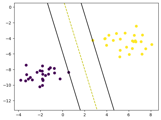

class SVMVectorized:
    def __init__(self, learning_rate=0.001, lambda_param=0.01, n_iters=1000):
        self.lr = learning_rate
        self.lambda_param = lambda_param
        self.n_iters = n_iters
        self.w = None
        self.b = None

    def fit(self, X, y):
        n_feats = X.shape[1]
        self.w, self.b = np.zeros(n_feats), 0
        y = np.where(y <= 0, -1, 1)
        
        for _ in range(self.n_iters):
            margins = y * (X @ self.w-self.b)
            misclassified = margins < 1 

            self.w -= self.lr*(2*self.lambda_param*self.w - np.dot(misclassified*y,X)) #correctly classified examples have hinge loss 0
            self.b -= self.lr*np.sum(misclassified*y)

    def predict(self, X):
        return np.sign(X @ self.w -self.b)

if __name__ == "__main__":
    # Imports
    from sklearn import datasets
    import matplotlib.pyplot as plt

    X, y = datasets.make_blobs(
        n_samples=50, n_features=2, centers=2, cluster_std=1.05, random_state=40
    )
    y = np.where(y == 0, -1, 1)

    clf = SVMVectorized()
    clf.fit(X, y)
    predictions = clf.predict(X)

    print(clf.w, clf.b)

    def visualize_svm():
        def get_hyperplane_value(x, w, b, offset):
            return (-w[0] * x + b + offset) / w[1]

        fig = plt.figure()
        ax = fig.add_subplot(1, 1, 1)
        plt.scatter(X[:, 0], X[:, 1], marker="o", c=y)

        x0_1 = np.amin(X[:, 0])
        x0_2 = np.amax(X[:, 0])

        x1_1 = get_hyperplane_value(x0_1, clf.w, clf.b, 0)
        x1_2 = get_hyperplane_value(x0_2, clf.w, clf.b, 0)

        x1_1_m = get_hyperplane_value(x0_1, clf.w, clf.b, -1)
        x1_2_m = get_hyperplane_value(x0_2, clf.w, clf.b, -1)

        x1_1_p = get_hyperplane_value(x0_1, clf.w, clf.b, 1)
        x1_2_p = get_hyperplane_value(x0_2, clf.w, clf.b, 1)

        ax.plot([x0_1, x0_2], [x1_1, x1_2], "y--")
        ax.plot([x0_1, x0_2], [x1_1_m, x1_2_m], "k")
        ax.plot([x0_1, x0_2], [x1_1_p, x1_2_p], "k")

        x1_min = np.amin(X[:, 1])
        x1_max = np.amax(X[:, 1])
        ax.set_ylim([x1_min - 3, x1_max + 3])

        plt.show()

    visualize_svm()

[0.60926001 0.16851888] -0.054000000000000034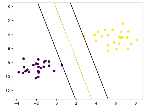

class SVMTorch(nn.Module):
    def __init__(self, input_dim, lambda_param=0.01):
        super().__init__()
        self.lin = nn.Linear(input_dim,1)
        self.lambda_param = lambda_param
    def forward(self, X):
        return self.lin(X)
    def hinge_loss(self, y_pred, y):
        h_loss = torch.mean(torch.clamp(1-y*y_pred,min=0))
        h_reg = self.lambda_param*0.5*torch.linalg.vector_norm(self.lin.weight, ord=2)**2
        return h_reg + h_loss

        


if __name__ == "__main__":
    # Imports
    from sklearn import datasets
    import matplotlib.pyplot as plt

    X, y = datasets.make_blobs(
        n_samples=50, n_features=2, centers=2, cluster_std=1.05, random_state=40
    )
    y = np.where(y == 0, -1, 1)
    X, y = torch.tensor(X, dtype=torch.float32), torch.tensor(y, dtype=torch.float32)

    # training loop
    n_iters, lr, lambda_param = 1000, 0.001, 0.01
    clf = SVMTorch(input_dim=X.shape[1], lambda_param=lambda_param)
    optimizer = torch.optim.SGD(params = clf.parameters(), lr=lr)
    for _ in range(n_iters):
        optimizer.zero_grad()
        y_pred = clf.forward(X).squeeze()
        loss = clf.hinge_loss(y_pred,y)
        loss.backward()
        optimizer.step()
    # preds
    with torch.no_grad():
        predictions = torch.sign(X @ clf.lin.weight.T - clf.lin.bias)

    print(clf.lin.weight, clf.lin.bias)

    def visualize_svm(X,y,clf):
        def get_hyperplane_value(x, w, b, offset):
            return (-w[0] * x + b + offset) / w[1]

        fig = plt.figure()
        ax = fig.add_subplot(1, 1, 1)
        X, y = X.cpu().numpy(), y.cpu().numpy()
        w, b = clf.lin.weight.cpu().detach().numpy().flatten(), clf.lin.bias.cpu().detach().numpy().flatten()
        plt.scatter(X[:, 0], X[:, 1], marker="o", c=y)
       
        x0_1 = np.amin(X[:, 0])
        x0_2 = np.amax(X[:, 0])

        x1_1 = get_hyperplane_value(x0_1, w, b, 0)
        x1_2 = get_hyperplane_value(x0_2, w, b, 0)

        x1_1_m = get_hyperplane_value(x0_1, w, b, -1)
        x1_2_m = get_hyperplane_value(x0_2, w, b, -1)

        x1_1_p = get_hyperplane_value(x0_1, w, b, 1)
        x1_2_p = get_hyperplane_value(x0_2, w, b, 1)

        ax.plot([x0_1, x0_2], [x1_1, x1_2], "y--")
        ax.plot([x0_1, x0_2], [x1_1_m, x1_2_m], "k")
        ax.plot([x0_1, x0_2], [x1_1_p, x1_2_p], "k")

        x1_min = np.amin(X[:, 1])
        x1_max = np.amax(X[:, 1])
        ax.set_ylim([x1_min - 3, x1_max + 3])

        plt.show()

    visualize_svm(X,y,clf)

Parameter containing:
tensor([[0.7446, 0.2005]], requires_grad=True) Parameter containing:
tensor([-0.3815], requires_grad=True)